Particle Wave Packets
A particle in free space who's momentum is known exactly can be described by the plane wave probability amplitude function:
Contents

where

 and
and
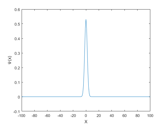
We will consider a particle that is localized in space with a Gaussian probabilty amplitude distribution at t=0 is:
Our appoach is to project this wave packet onto the plane wave solutions, then let each plane wave evolve as $e^{i( k x - \omega t)}%
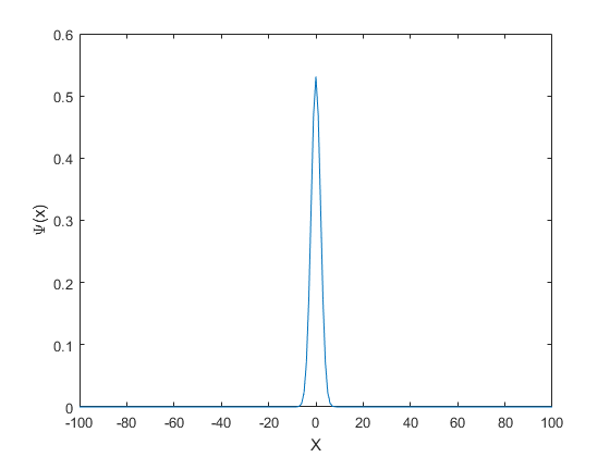
Lets make a wave packet
Lets take hbar=1, m=1
N=201;
X=linspace(-100,100,N);
DX=X(2)-X(1);
Sigma=2;
A=normpdf(X,0,Sigma);
A=A/sqrt(A*A'*DX); %Normalize
figure
plot(X,A)
xlabel('X');ylabel('\Psi(x)')
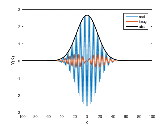
Write wave packet as a sum of plane waves
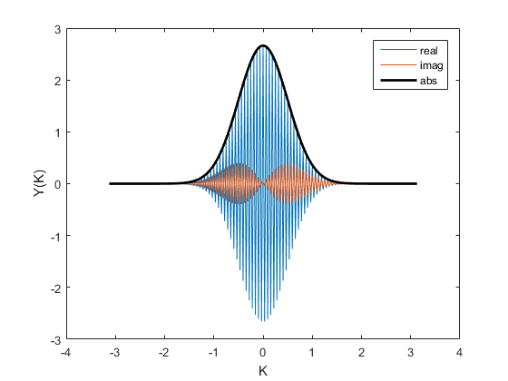
% Expanding into plane waves is just the Fourier transform:
Y=fftshift(fft(A));
K=(0:N-1);
K(K>N/2)=K(K>N/2)-N;
K=fftshift(K);

% Plot the wave in k-space (this is spatial frequency)
figure
plot(K,real(Y))
hold
plot(K,imag(Y))
plot(K,abs(Y),'k','linewidth',2)
legend('real','imag','abs')
xlabel('K');ylabel('Y(K)')
% Note the magnitude of the Y(k) is also a Gaussian.
% The FT of a Gaussian is a Gaussian.
% web('http://mathworld.wolfram.com/FourierTransformGaussian.html')


% Plot as wave number with correct units
figure
DK=1/(N*DX);
KWV=2*pi*K*DK;     %Wave number
plot(KWV,real(Y))
hold
plot(KWV,imag(Y))
plot(KWV,abs(Y),'k','linewidth',2)
legend('real','imag','abs')
xlabel('K');ylabel('Y(K)')
Current plot held
Current plot held
Now let's reconstruct the wave from Fourier coefficients at t=0
close all
Wave=0
figure
for kk=1:N
    KS=K(kk);           %Spatial frequency
    KWV=2*pi*KS;        %Wave number
    PlaneWave=1/N*exp(i*KWV*(0:N-1)/N);
    Wave=Wave+Y(kk)*PlaneWave;
    plot(X,real(Wave))
    xlabel('X');ylabel('\Psi(x)')
    pause(.01)
end
Wave =

     0
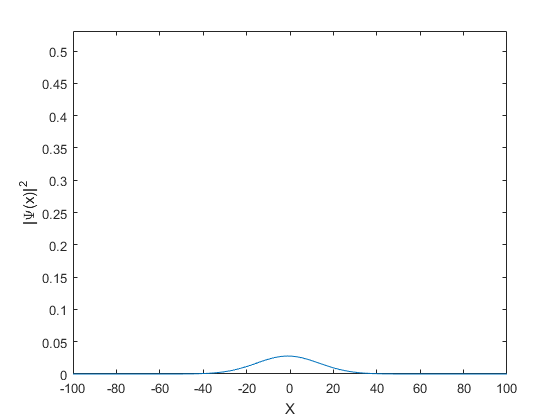
Now let's look at time evolution
Tvec=linspace(0,.001,100);
figure
for tt=1:length(Tvec)
    Wave=0;
    t=Tvec(tt);
    for kk=1:N
        KS=K(kk);           %Spatial frequency
        KWV=2*pi*KS;        %Wave number
        W=1/2*KWV^2;        %Omega
        PlaneWave=Y(kk)/N*exp(i* (KWV/N*(1:N)-W*t) );
        Wave=Wave+PlaneWave;
    end
    plot(X,abs(Wave).^2)
    axis([-100 100 0 max(A)])
    xlabel('X');ylabel('|\Psi(x)|^2')
    pause(.01)
end